Prerequisito: Regressione lineare
La regressione lineare è un algoritmo di machine learning basato sull'apprendimento supervisionato. Esegue un'attività di regressione. La regressione modella un valore di previsione target basato su variabili indipendenti. Viene utilizzato principalmente per scoprire la relazione tra variabili e previsioni. Diversi modelli di regressione differiscono in base al tipo di relazione tra le variabili dipendenti e indipendenti che stanno considerando e al numero di variabili indipendenti utilizzate. Questo articolo dimostrerà come utilizzare le varie librerie Python per implementare la regressione lineare su un determinato set di dati. Dimostreremo un modello lineare binario poiché sarà più facile da visualizzare. In questa dimostrazione, il modello utilizzerà Gradient Descent per apprendere. Puoi scoprirlo qui.
Passo 1: Importazione di tutte le librerie richieste
Python3
import> numpy as np> import> pandas as pd> import> seaborn as sns> import> matplotlib.pyplot as plt> from> sklearn>import> preprocessing, svm> from> sklearn.model_selection>import> train_test_split> from> sklearn.linear_model>import> LinearRegression> |
>
>
la migliore macchina del mondo
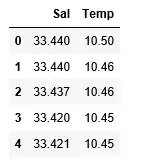
Passo 2: Lettura del set di dati:
Python3
df>=> pd.read_csv(>'bottle.csv'>)> df_binary>=> df[[>'Salnty'>,>'T_degC'>]]> > # Taking only the selected two attributes from the dataset> df_binary.columns>=> [>'Sal'>,>'Temp'>]> #display the first 5 rows> df_binary.head()> |
>
>
Produzione:
Passaggio 3: Esplorare la dispersione dei dati
Python3
divisione delle stringhe c++
#plotting the Scatter plot to check relationship between Sal and Temp> sns.lmplot(x>=>'Sal'>, y>=>'Temp'>, data>=> df_binary, order>=> 2>, ci>=> None>)> plt.show()> |
>
>
Produzione:

Passaggio 4: Pulizia dei dati
Python3
# Eliminating NaN or missing input numbers> df_binary.fillna(method>=>'ffill'>, inplace>=> True>)> |
>
>
Passaggio 5: Addestrare il nostro modello
Python3
X>=> np.array(df_binary[>'Sal'>]).reshape(>->1>,>1>)> y>=> np.array(df_binary[>'Temp'>]).reshape(>->1>,>1>)> > # Separating the data into independent and dependent variables> # Converting each dataframe into a numpy array> # since each dataframe contains only one column> df_binary.dropna(inplace>=> True>)> > # Dropping any rows with Nan values> X_train, X_test, y_train, y_test>=> train_test_split(X, y, test_size>=> 0.25>)> > # Splitting the data into training and testing data> regr>=> LinearRegression()> > regr.fit(X_train, y_train)> print>(regr.score(X_test, y_test))> |
>
>
Produzione:

Passaggio 6: Esplorando i nostri risultati
Python3
alfabeto ai numeri
y_pred>=> regr.predict(X_test)> plt.scatter(X_test, y_test, color>=>'b'>)> plt.plot(X_test, y_pred, color>=>'k'>)> > plt.show()> # Data scatter of predicted values> |
>
>
Produzione:

Il basso punteggio di accuratezza del nostro modello suggerisce che il nostro modello regressivo non si adatta molto bene ai dati esistenti. Ciò suggerisce che i nostri dati non sono adatti per la regressione lineare. Ma a volte un set di dati può accettare un regressore lineare se ne consideriamo solo una parte. Verifichiamo questa possibilità.
Passaggio 7: Lavorare con un set di dati più piccolo
Python3
df_binary500>=> df_binary[:][:>500>]> > # Selecting the 1st 500 rows of the data> sns.lmplot(x>=>'Sal'>, y>=>'Temp'>, data>=> df_binary500,> >order>=> 2>, ci>=> None>)> |
>
>
Produzione:

Possiamo già vedere che le prime 500 righe seguono un modello lineare. Proseguendo con gli stessi passaggi di prima.
Python3
df_binary500.fillna(method>=>'fill'>, inplace>=> True>)> > X>=> np.array(df_binary500[>'Sal'>]).reshape(>->1>,>1>)> y>=> np.array(df_binary500[>'Temp'>]).reshape(>->1>,>1>)> > df_binary500.dropna(inplace>=> True>)> X_train, X_test, y_train, y_test>=> train_test_split(X, y, test_size>=> 0.25>)> > regr>=> LinearRegression()> regr.fit(X_train, y_train)> print>(regr.score(X_test, y_test))> |
>
>
Produzione:
Java se altro

Python3
y_pred>=> regr.predict(X_test)> plt.scatter(X_test, y_test, color>=>'b'>)> plt.plot(X_test, y_pred, color>=>'k'>)> > plt.show()> |
>
>
Produzione:

Passaggio 8: Metriche di valutazione per la regressione
Infine, controlliamo le prestazioni del modello di regressione lineare con l'aiuto di metriche di valutazione. Per gli algoritmi di regressione utilizziamo ampiamente le metriche mean_absolute_error e mean_squared_error per verificare le prestazioni del modello.
Python3
from> sklearn.metrics>import> mean_absolute_error,mean_squared_error> > mae>=> mean_absolute_error(y_true>=>y_test,y_pred>=>y_pred)> #squared True returns MSE value, False returns RMSE value.> mse>=> mean_squared_error(y_true>=>y_test,y_pred>=>y_pred)>#default=True> rmse>=> mean_squared_error(y_true>=>y_test,y_pred>=>y_pred,squared>=>False>)> > print>(>'MAE:'>,mae)> print>(>'MSE:'>,mse)> print>(>'RMSE:'>,rmse)> |
>
>
Produzione:
MAE: 0.7927322046360309 MSE: 1.0251137190180517 RMSE: 1.0124789968281078>